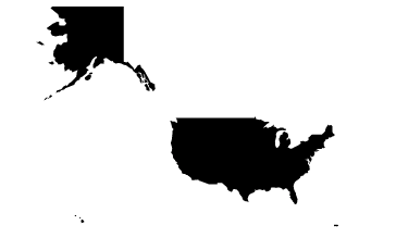
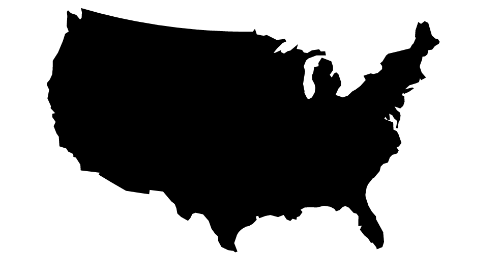
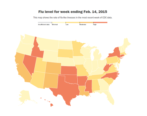
Stephen and Danny's D3 Mapping Presentation

class: center, middle
name: how
layout: false

# Stephen and Danny's D3 Mapping Presentation:
![googlemap](https://raw.githubusercontent.com/stat4701-edav-d3/stat4701-edav-d3.github.com/master/remark-develop/img/googlemap.jpg) 
## A Crash Course from Shapefile to TopoJSON (and some GeoJSON) using GDAL/OGR

---

.left-column[
  #Agenda
]

.right-column[
  ## Introduction
  ## Getting a Shapefile
  ## Conversion
  ## Plotting the JSON in D3
  ## Shapefile vs. GeoJSON vs. TopoJSON 
  ## Flu Data
  ## Demo: Choropleth
  ## Demo: Interactive Map (Tom Noda)
  ## Demo: Google Flu Data Map
]
---

.left-column[
  # Introduction
]

.right-column[

* ##About Us
  * ####Stephen
  * ####Danny

* ##Familiarity with JavaScript and D3?

* ##Why we picked this topic? 
  * ####Get more familiar with JavaScript and D3

* ##What to expect? 
  * Some maps
  * Some live D3 demos
  * and...

some code

]

---

# Getting a Shapefile

## Downloading the Shapefile
  ####[From the United States Census Bureau](https://www.census.gov/geo/maps-data/data/tiger-line.html)
  ```js
  import urllib

zipLoc = "/data/cb_2013_us_state_20m.zip"
  fileURL = "http://www2.census.gov/geo/tiger/GENZ2013/cb_2013_us_state_20m.zip"
  urllib.urlretrieve (fileURL, zipLoc) #get that file

import zipfile  
  
  zip = zipfile.ZipFile(zipLoc)  
  zip.extractall("/data/census/states/") #unzip!

```

---

# The Shapefile 
  #### What's with all these files?

* .shp—The main file that stores the feature geometry; required.

* .shx—The index file that stores the index of the feature geometry; required.

* .dbf—The dBASE table that stores the attribute information of features; required. There is a one-to-one relationship between geometry and attributes, which is based on record number. Attribute records in the dBASE file must be in the same order as records in the main file.

* .sbn and .sbx—The files that store the spatial index of the features.

* .prj—The file that stores the coordinate system information; used by ArcGIS.

* .xml—Metadata for ArcGIS—stores information about the shapefile.

---
  # The Shapefile 
  #### What's with all these files? 
optional files:

* .fbn and .fbx—The files that store the spatial index of the features for shapefiles that are read-only.

* .ain and .aih—The files that store the attribute index of the active fields in a table or a theme's attribute table.

* .atx—An .atx file is created for each shapefile or dBASE attribute index created in ArcCatalog. ArcView GIS 3.x attribute indexes for shapefiles and dBASE files are not used by ArcGIS. A new attribute indexing model has been developed for shapefiles and dBASE files.

* .ixs—Geocoding index for read/write shapefiles.

* .cpg—An optional file that can be used to specify the codepage for identifying

* .mxs—Geocoding index for read/write shapefiles (ODB format).

---

#[IPython Notebook: The Setup and Download and Unzip a Shapefile](http://nbviewer.ipython.org/github/stat4701-edav-d3/d3-presentation/blob/master/00-d3-presentation.ipynb#The-Setup)

---

.left-column[
  #Conversion
]

.right-column[
  ##GDAL/OGR
  Now that we have our Shapefile, we need to convert it into JSON in order to use it in web applications. This is a two-step process -- we will convert .shp into GeoJSON and then convert GeoJSON into Topojson using a few nifty tools.

* ###GDAL - Geospatial Data Abstraction Library - Raster Data
  *It is sometimes pronounced "goo-doll" (a bit like goo-gle), while others pronounce it "gee-doll," and others pronounce it "gee-dall."*

* ###OGR - formerly known as OpenGIS Simple Features Reference Implementation - Vector Data
  *OGR used to stand for OpenGIS Simple Features Reference Implementation. However, since OGR is not fully compliant with the OpenGIS Simple Feature specification and is not approved as a reference implementation of the spec the name was changed to OGR Simple Features Library. The only meaning of OGR in this name is historical. OGR is also the prefix used everywhere in the source of the library for class names, filenames, etc.*

**Both of these definitions are from [OSGEO FAQ](https://trac.osgeo.org/gdal/wiki/FAQGeneral)**
]

---
.left-column[
 # Shapefile vs. GeoJSON vs. TopoJSON 
]
.right-column[

#Comparing file sizes of the same features represented in a Shapefile, GeoJSON and a TopoJSON file. 
![full-col-width](http://commondatastorage.googleapis.com/imgserv%2Ffilesize.png)
]

---

.left-column[
  #Conversion
]

.right-column[

##Shapefile to GeoJSON
  For this first step, we're going to use [GDAL/OGR](http://www.gdal.org/). GDAL/OGR can be installed using ```sudo apt-get install gdal-bin``` 
  or, for all you OSX folks, ```brew install gdal```.

Next, using the ```ogr2ogr``` commands, we can convert the Shapefile to JSON:

ogr2ogr -f GeoJSON states.json cb_2013_us_state_20m.shp

]

---

.left-column[
  #Conversion
]
.right-column[

##GeoJSON to TopoJSON

For the next step, we need to install topojson. Before doing this though, you need to make sure youhave [node.js](http://nodejs.org/download/) installed.

Using the command ```sudo npm install -g topojson``` or ```sudo npm install -g topojson``` (OSX) will then install topojson. We can then create our TopoJson:

topojson -o states_topo.json states.json
]

---

###Another Option, as you may want to modify and tweak the Simplification algorithm of the TopoJson file, is...
#MapShaper

* ##[MapShaper](http://www.mapshaper.org/)

* ##Demo MapShaper with Census Shapefile on Desktop

---

.left-column[
 #Plotting in D3
]
.right-column[

###[The TopoJSON file in a simple plot](http://stat4701-edav-d3.github.io/viz/plot_json_1.html)






 [![plot json](https://raw.githubusercontent.com/stat4701-edav-d3/d3-presentation/master/img/plot_json.png)](http://stat4701-edav-d3.github.io/viz/plot_json_1.html)

###[Here’s the HTML code](https://github.com/stat4701-edav-d3/stat4701-edav-d3.github.com/blob/master/viz/plot_json_1.html)

]
---

##That's enough to make you want to install a local instance of cold beer.

![cold beer](https://camo.githubusercontent.com/9dd59c598e38baf943174ad4cb2d334401ba8a34/687474703a2f2f746865736f636965747970616765732e6f72672f736f63696d616765732f66696c65732f323031302f30382f70616273742d626c75652d726962626f6e2e6a7067)

*image inspired by CartoDB install instructions*

However, that is hardly a presentable map...

---

.left-column[
  #Plotting the JSON in D3
]
.right-column[

#Reconfiguring the Map Extents

[The Map with new Extents](http://stat4701-edav-d3.github.io/viz/plot_json_2.html)

![full-col-width](http://raw.githubusercontent.com/stat4701-edav-d3/d3-presentation/master/img/json_albers.png)

[Here’s the HTML code - Project to albers](https://github.com/stat4701-edav-d3/stat4701-edav-d3.github.com/blob/master/viz/plot_json_2.html)
]

---

#What to map?

####We wanted to map some data that seemed interesting.

#We had a few ideas to map **Flu** data

* ##Sources of Flu Data
  * ###CDC Flu Data
    * [R script for CDC Flu Data and Basic Munging](https://github.com/stat4701-edav-d3/stat4701-edav-d3.github.com/blob/master/flu_eda.R)

* ###Google Flu Trends
    * [IPython Notebook of Google Flu Trends Data](http://nbviewer.ipython.org/github/stat4701-edav-d3/d3-presentation/blob/master/00-d3-presentation.ipynb#The-Google-Flu-Data)

* ###Why?...

---

.left-column[
  # Demo: Google Flu Data Map
]

.right-column[

The vaccine for the 2014-2015 flu season has only been [18% effective](http://www.nlm.nih.gov/medlineplus/news/fullstory_151174.html) against the dominant strain (H3N2) of the flu. 
  There have already been some great visualizations of flu data including the Washington Post's weekly [flu tracker](http://www.washingtonpost.com/graphics/health/flu-tracker/):

![WaPo Flu](https://raw.githubusercontent.com/stat4701-edav-d3/stat4701-edav-d3.github.com/master/remark-develop/wapo.jpg)

]

---
.left-column[
 # Demo: Choropleth
]
.right-column[

#[Link to Choropleth of Flu Data by State](http://stat4701-edav-d3.github.io/viz/choropleth/choropleth.html)

#[The Choropleth of Flu Data by State HTML code](https://github.com/stat4701-edav-d3/stat4701-edav-d3.github.com/blob/master/viz/choropleth/choropleth.html)

###[The Flu data split by week and normalized by State population (rate per 10,000) - assigned to county, not distrubuted, for joining purposes to the json file we had.](https://github.com/stat4701-edav-d3/stat4701-edav-d3.github.com/tree/master/viz/choropleth/data)
This example was heavily inspired by [Mike Bostock's Let's Make a Map](http://bost.ocks.org/mike/map/).

]

---

.left-column[
  # Demo: Google Flu Data Map
]

.right-column[

## Munging the Data:

### [IPython Notebook: Geocoding the Cities with Nominatim](http://nbviewer.ipython.org/github/stat4701-edav-d3/d3-presentation/blob/master/02-cities-to-cartodb.ipynb)
  * [Nominatim Geocoder](http://wiki.openstreetmap.org/wiki/Nominatim)

### [IPython Notebook: Munging and combining weeks into years](http://nbviewer.ipython.org/github/stat4701-edav-d3/d3-presentation/blob/master/04-format-cities-for-map.ipynb)

]
---

.left-column[
  # Demo: Google Flu Data Map
]

.right-column[

## Visualizing Cities Flu Data

### [Visualizing the Flu: Google Flu Trends in D3.js (September 2003 - March 2015)](http://stat4701-edav-d3.github.io/viz/cities/cities.html)
* Inspired and hacked from [@AxisMaps](https://twitter.com/axismaps) [Geography of Jobs](http://tipstrategies.com/geography-of-jobs/).

]
---

.left-column[
  # Demo: Interactive Map
]

# Interactive Map with d3.js

One of [Tom Noda's Maps](http://www.tnoda.com/blog/2013-12-07) heavily inspired a lot what we **tried** to do. But couldn't quite get. So we thought we'd share it with you. We even had trouble just getting this to run locally and on our site.

[Interactive Map with d3.js](http://stat4701-edav-d3.github.io/tnoda/index.html)